Machine learning over the p-adics
A brief introduction to non-Archimedean optimisation
Joint work with Yiannis Fam, Anthea Monod and Yue Ren.
Table of contents
-
Some background about ML & motivation
-
Polydisc spaces
-
Optimisation on polydisc spaces
-
Applications
Machine learning, in brief
Usual setup in machine learning:
Data
-
Inputs:
x_1, \ldots, x_n \in \RR^d -
Outputs:
y_1, \ldots, y_n \in \RR^e
For example, x_i could describe a house and y_i its price,
or x_i could be a picture and y_i indicate whether it contains a kitten.

y_1 = 1

y_2 = 0
Goal: “learn” the relation between the x_i and the y_i.
The machine-learning recipe
-
(Model) Choose a parametrised family of functions:
f_\theta : \RR^d \to \RR^eHere\thetais the parameter, and we wantf_\theta(x_i) \approx y_i. -
(Data) Create a dataset of examples
(\mathbf{x}, \mathbf{y}) = \{(x_i, y_i)\}_{i=1}^n. -
(Loss) Choose a loss function
\ell(\theta) = \ell(\theta; \mathbf{x}, \mathbf{y}) -
(Optimisation) Find a parameter
\thetathat minimises the loss.
Example: regression
-
Model: E.g.
f_\theta(x) = Ax + b(or something more complicated) -
Parameter:
\theta = \{A, b\} -
Loss:
\ell(\theta; \mathbf{x}, \mathbf{y}) = \sum_{i=1}^{n}
  |y_i - f_\theta(x_i)|^2
Neural networks
Example. A neural network is a function of the form
f_\theta(x) = \sigma \circ L_d \circ \sigma \circ L_{d-1}
\circ \cdots \circ L_1(x)
where each L_i is an affine map and \sigma is non-linear, for example
\sigma(t) = \max(0,t)
or
\sigma(t) = \frac{1}{1+e^{-t}}.
Optimisation (minimisation of the loss)
We can view loss minimisation as the gradient-flow ODE
\frac{d\theta}{dt} = - \nabla_\theta \ell(\theta)
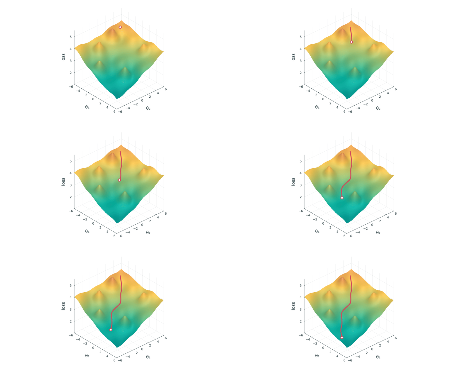
In practice, we discretise this to get the gradient-descent algorithm.
Gradient descent
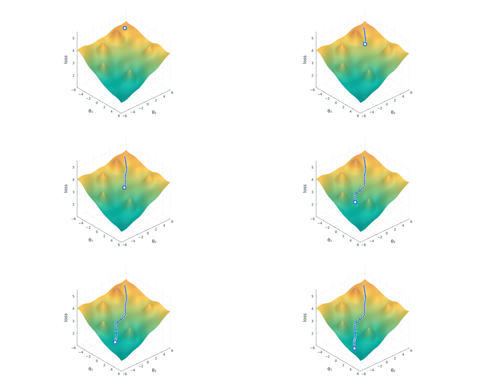
Classical gradient descent
Algorithm:
-
Pick an initial parameter
\theta=\theta_0 \in \RR^n. -
For
n=0,1,2,\ldots, repeat: -
Compute
\nabla_\theta fat\theta_n. -
Set
\theta_{n+1}to be\theta_n-\alpha\nabla f(\theta_n). -
Go back to step 2.
In practice: \nabla f is computed by backpropagation using specialised hardware (GPUs, TPUs, etc.).
If f is complicated, this can be expensive.
What about the p-adics?
Why do we care?
- Maths
- Useful for computations.
- Interesting theoretical questions about algorithms.
- ''Learning'' mathematical invariants and formulating conjectures. E.g. murmurations of elliptic curves, etc.
- Fun example: solving systems of polynomials.
- Applications
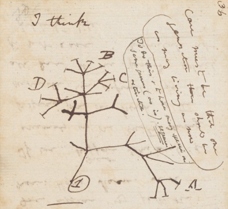
- Hierarchical data is non-Archimedean
What about the p-adics?
What changes?
-
\QQ_pis not path-connected; in fact it is totally disconnected. -
We can have locally constant functions which are not constant.
-
We don't have a good notion of gradient.
Non-Archimedean geometry
-
(closed) points on
\BA^n_Kare homomorphismsK[T_1, \ldots, T_n] \to K. -
The Berkovich affine space
\BA^n_{\mathrm{Berk},K}is the set of multiplicative seminorms|\cdot| : K[T_1, \ldots, T_n] \to \RR_{\geq 0}extending the norm onK. -
(there is a more general notion of Berkovich analytic spaces)
Example
If
a \in \CC_p^nandr \in \RR_{\geq 0}^n, we can define the multiplicative seminorm| \cdot | _{B(a,r)} : \QQ_p[T_1, \ldots, T_n] \to \RR_{\geq 0}via|f|_{B(a,r)} \coloneqq \sup_{z \in B(a,r)} |f(z)|_K.
Here, B(a,r) is the closed polydisc in \CC_p^n of radius r around a.
One can check that
|f|_{B(a,r)} = \sup_{\alpha \in \N^n} |c_\alpha| r^\alpha,wheref = \sum_\alpha c_\alpha (T-a)^\alpha.
When r = 0 this is evaluation at a point.
Berkovich spaces
-
Berkovich spaces can be defined in general by gluing affinoid spaces.
-
These are the analogues of affine schemes in scheme theory.
-
For a variety
Xover\hat K, we can define the Berkovich analytificationX^{\an}. -
There are comparison theorems for the étale cohomology of
XandX^{\an}.
The Berkovich affine line
Berkovich's Classification Theorem:
The discs
B(a,r) \subset \CC_p, witha \in \CC_pandr \geq 0, are almost all the points of\BA^1_{\mathrm{Berk},\CC_p}.
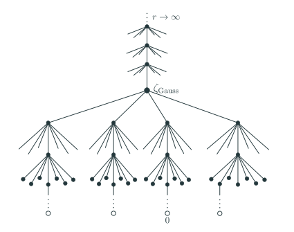
Branching happens when r \in | \CC_p^\times | = p^{\QQ} (''rational points'').
Remarks
-
Over
\CC_p, rational points on the affine line have infinitely many branches. This is not practical for computation. -
The situation is much worse in higher dimensions: no such explicit description of the points of
\BA^n_{\mathrm{Berk},\CC_p}. -
In practice, we want to work with smaller fields, such as
\QQ_p, and a subset\BB^n \subset \BA^n_{\mathrm{Berk},\CC_p}.
Polydisc space - Definition
Definition: The
n-polydisc space is
\BB^n(\QQ_p)\coloneqq\left\{
    B(a_1,r_1)\times\cdots\times B(a_n,r_n)
    :a_i\in\QQ_p,\ r_i\in\RR_{\geq 0}\right\}.
This has a natural topology, and several natural metrics.
If for all i, we have r_i \in p^\ZZ then say that the polydisc is rational.
Polydisc space - Definition
Example (\BB^1 for p=2)
Polydisc space - Metric
Absolute and valuative metrics (\BB^1 for p=2)
Field extensions reshape disc spaces
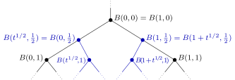
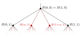
For a valued field extension K\subseteq L, the inclusion
B_K(a,r)\longmapsto B_L(a,r) embeds \BB^1(K) in \BB^1(L).
\mathbb F_2((t))\subseteq\mathbb F_2((t^{1/2}))
\mathbb F_2((t))\subseteq\mathbb F_4((t))
3 becomes degree 5.
Polydisc space - Functions
Definition (absolute polynomials)
Any polynomial f\in\QQ_p[x_1,\ldots,x_n] gives a continuous real-valued function
|f|:\BB^n\longrightarrow\RR_{\geq 0},\qquad
  B\longmapsto |f|_B\coloneqq\sup_{z\in B}|f(z)|_p.
-
|f|is piecewise polynomial in the radius. -
|f|is monotone:|f|_B\leq |f|_{B'}wheneverB\subseteq B'. -
a_1|f_1|+\cdots+a_r|f_r|, witha_i\in\RR, are universal approximators. -
These sums often have global minima (related to the projective hypersurfaces defined by
the
f_i).
f(T)=T^2-1
over
\QQ_2.
|T^2-1|_{B(1,r)}=\frac r2.
|T^2-1|_{B(-1,r)}=\frac r2.
Doing optimisation in practice
Julia library: NonArchimedeanMachineLearning.jl
p\gg 0 large
continuous optimisation
p>0 small
combinatorial optimisation




Tree search
If we restrict to polydiscs with rational radii, minimisation becomes a tree search problem.
These are well-studied problems in computer science!
These come in several forms:
-
deterministic
-
stochastic
Goal: explore the tree in a way that finds a minimum quickly.
Design tradeoff: need to
-
explore enough that we don't miss a minimum, but
-
avoid exploring too much and wasting time on unpromising branches.
Optimising over polydiscs is like playing chess
Computer chess: need to explore the tree of possible moves:
-
explore enough that we don't miss a good move, but
-
avoid exploring too much and wasting time on unpromising moves.
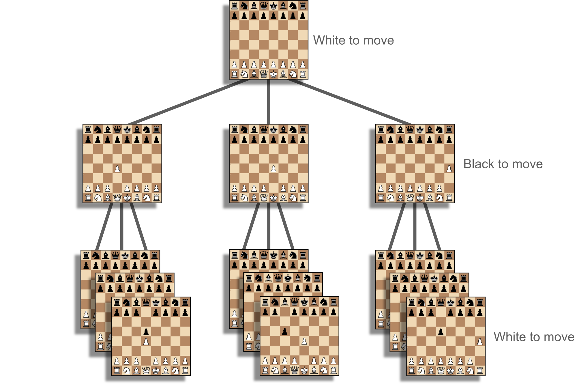
We can adapt one of the most successful chess algorithms, Monte Carlo tree search (MCTS).
Monte Carlo tree search, in brief
Key idea: give each node P a score (updated over time), and explore the most promising nodes first.
\begin{aligned}
\mathrm{score}(P)
  &= \text{current estimated value of }P\\
  &\quad + \text{exploration bonus for }P.
\end{aligned}
For each node P we associate some statistics:
-
the number of times it has been visited:
N_{\text{visits}}(P) -
the average value (or maximum) of
fat its children:Q(P)
The current estimated value and the exploration bonus are functions of these.
Monte Carlo tree search
One MCTS iteration:
-
Start at the root.
-
Select the best-scoring child until we reach a leaf.
-
Evaluate
fat that leaf. -
Expand the leaf by adding its children.
-
Update scores along the path, then return to the root.
Solving polynomials
We can use this to produce approximations to the roots of polynomials over valued fields K.
Let f \in K[x_1, \dots, x_n] be a polynomial. We want to find a \in K^n such that
f(a)=0 (if it exists).
As a minimisation problem:
\mathrm{argmin}_{a \in K^n} |f(a)|.
This naturally extends to the polydisc space \BB^n:
\mathrm{argmin}_{P \in \BB^n} |f(P)|.
A root corresponds to the global minimum value 0.
MCTS for ''solving'' a polynomial equation
Toy examples: let f(P) = |T^2-1|_P.

Running algorithms on this
-
Algorithms that provably converge can approximate roots of polynomials over valued fields.
-
The same approach extends to systems of polynomials and more general functions.
-
The rate of convergence appears to be related to the sizes of tubular neighbourhoods of the hypersurfaces defined by the polynomials.
What’s next?
-
Theoretical: interesting mathematical questions about algorithms.
-
Test these techniques with more real-world data.
-
Benchmark the algorithms: are non-Archimedean techniques faster than the alternatives?
-
What other classes of functions might we want to optimise?